In this guide I first review the intuition of Monte Carlo methods, and then discuss five steps to efficient, publication-quality Monte Carlo analyses using R. Generally, these steps consist of:

Switching from serial to parallel loops
Ensuring reproducibility by setting seeds properly for parallel tasks
Ensuring that other parallel tasks are not competing for CPU resources
Properly setting up simulation parameter grids
Compartmentalizing code into simulation and estimation functions
A few dos and don’ts

First, I will walk through each of these five points with toy examples to drive ideas home where applicable. Finally, I will take all of this and put it together in some more serious applications.

Note that this guide applies mostly to the case of trivial parallelism, i.e., simulations that are independent of each other. However, some concepts can be extended to dependent simulations, particularly in MCMC algorithms that rely on full-conditionals. Where this is the case, I note it in the Caveats subsection of a topic.

1 Brief Review of Monte Carlo Methods

The goal of Monte Carlo analysis is to investigate the behavior of a statistic using an approximation of its sampling distribution. All of Monte Carlo analysis then hinges on a Law of Large numbers. These laws effectively state that the sample mean of a random variable converges to its population mean, i.e., that the sample mean is a consistent estimator. With that idea in mind, we can also compute a whole host of other interesting quantities, such as the variance, the density function, or the quantile function, because all of these can be re-written as a sample mean of a random variable. Without any math, this is the primary intuition of Monte Carlo analysis: many of the quantities that we are interested in can be expressed as a sample mean of a random variable, so we know they converge to the true value of the quantity of interest due to a law of large numbers.

For example \[ \lim_{n\to\infty} \frac{1}{n}\sum_{i=1}^n X_i = \mu_x \] meaning that the sample mean converges to the population mean as the sample size tends to infinity. However, as the bold text above indicates, a whole host of other quantities converge to their true expected values, for example:

The variance:¹ \[\frac{1}{n} \sum_{i=1}^n (X_i - \bar X)^2 \longrightarrow \mathrm{var}(X)\]
The CDF: \[\hat F(x) = \frac{1}{n} \sum_{i=1}^n \underset{(-\infty, x]}{\mathbb{I}}(X_i) \longrightarrow F_X(x)\]
The density function (using kernel $K$ and bandwidth $h$):² \[\hat f(x) = \frac{1}{n} \sum_{i=1}^{n} \frac{1}{h} K\left(\frac{x - X_i}{h}\right) \longrightarrow f_X(x)\]
The quantile function:³ \[\hat Q\{\hat F(x)\} = \text{inf}\left\{x:\frac{1}{n}\sum_{i=1}^{n}\underset{(-\infty, x]}{\mathbb{I}}(X_i) \geq \alpha)\right\} \longrightarrow \text{inf}\{x: F_X(x) \geq \alpha\}\]

So effectively we can simulate random variables, compute some function of those realizations, then take the mean of the resulting quantity, and the WLLN tells us that we converge to the expected value of that function.

Show me the math

To prove the WLLN, we will need a a few pieces of background information, namely Markov’s Inequality (used only to prove Chebyshev’s), Chebyshev’s inequality, and the definition of convergence in probability (note that all of this information can also be found in most math-stat textbooks, or on Wikipedia).

Markov’s Inequality: Let $X$ be a random variable with support over the non-negative real line, i.e., $\Pr(X \geq 0) = 1$. Then for every number $c > 0$, $\,\,\Pr(X \geq c) \leq \frac{\mathbb{E}(X)}{c}$.

Proof
Assuming continuous $X$ with pdf $f$: \[\begin{align*} \mathbb{E}(X) &= \int_0^\infty x f(x) \,dx \\ &= \int_0^c x f(x) \,dx + \int_c^\infty x f(x) \,dx \\ &\geq \int_0^c x f(x) \,dx + \int_c^\infty c f(x) \,dx \\ &= \int_0^c x f(x) \,dx + c \int_c^\infty f(x) \,dx \\ &= c \Pr(X \geq c) + \int_0^c x f(x) \,dx\\ &\geq c\Pr(X \geq c) \\[1em] \implies \Pr(X \geq c) &\leq \frac{\mathbb{E}(X)}{c} \end{align*}\]

Chebyshev’s Inequality: Let $X$ be a random variable with finite first and second moments, $\mu_X < \infty$ and $\sigma^2_X < \infty$ respectively. Then for all numbers $c > 0$, $\,\, \Pr(|X - \mu_X| \geq c) \leq \frac{\sigma^2_X}{c^2}$
Proof

Let $Y = (X - \mu_X)^2$ and $c^2 = k$, then:
- $\Pr(|X - \mu_X| \geq c) = \Pr\left[(X-\mu_X)^2 \geq c^2\right] = \Pr(Y \geq k)$, and
- $\mathbb{E}(Y) = \mathbb{E}\left[(X - \mu_X)^2\right] = \sigma^2_X$ by definition.
- Then by Markov’s Inequality, we have: \[\Pr(|X - \mu_X| \geq c) = \Pr(Y \geq k) \leq \frac{\mathbb{E}(Y)}{k} = \frac{\sigma^2_X}{c^2}\]

Convergence in Probability (to a constant): For a sequence of independent random variables $X_n = X_1, X_2, ...$ with the same mean $\mu_X < \infty$ and same variance $\sigma^2_X < \infty$, and for constants $c$ and $\varepsilon$: if $\lim_{n\to\infty} \Pr(|X_n - c|>\varepsilon) = 0 \hspace{1em} \forall \hspace{1em} \varepsilon > 0$ then $\,\,X_n \overset{p}{\longrightarrow} c$.

The WLLN then states that

\[\begin{equation*}\frac{1}{n} \sum_{i=1}^{n} X_i \overset{p}{\longrightarrow} \mu_X \end{equation*}\]

which can be generalized to functions $g$ of $X$:

\[\begin{equation*} \lim_{n\to\infty} \frac{1}{n}\sum_{i=1}^n g(X_i) \overset{p}\longrightarrow \mathbb{E}[g(X_n)] = \int_{X} g(x) \,\, \mathrm dF_X(x) \end{equation*}\]

for random variables $X_i \overset{iid}{\sim} f_X, \,\, i\in 1,2,...,n$, and (almost) any function $g$. This effectively says that the sample average of nearly any function of the data converges in probability to the true expected value.

This is proven using Chebyshevs inquality. First, by the linearity of expectation, we know that $\mathbb{E}(\bar X) = \mu_X$ and $\mathrm{var}(\bar X) = \sigma^2_X/n$. Then,

\[\begin{align*} \Pr(|\bar X - \mu_X| \geq \varepsilon) &\leq \frac{\sigma^2_X}{n\varepsilon^2} \\[1ex] \implies \lim_{n\to\infty} \Pr(|\bar X - \mu_X| \geq \varepsilon) &\leq \lim_{n\to\infty} \frac{\sigma^2_X}{n\varepsilon^2} \\[1em] &= 0 \end{align*}\] where this last equality follows because $0 \leq \lim_{n\to\infty} \Pr(|\bar X - \mu_X| \geq \varepsilon) \leq 0$ by the definition of a density function for the lower bound, which concludes the proof.

2 Simulations: Serial vs Parallel

As implied by the review of Monte Carlo analysis, simulations will involve a great number of iterations in order to obtain a sufficiently large sample to be averaged over, such that the error in our approximation is small (as we’ll never actually have infinite simulations). Unfortunately, R is single-threaded by default, meaning everything that you do in R is executed on a single CPU on your computer. So even if you have a quad-core processor that has 8 CPUs due to multi-threading, only one of these 8 potential processes is being used by R by default. However, given the fact that we’ll be doing a lot of simulation iterations, most Monte Carlo analyses would theoretically benefit from being able to compute quantities simultaneously: if we want to compute a bunch of sample means that are independent of eachother, then why not compute 8 means at a time, rather than one at a time? Naturally then, implementing Monte Carlo analyses in parallel will be the first step to obtaining results efficiently. There are exceptions to this rule (e.g., reserving computing resources for other tasks, parallel overhead making things slower), but if the reason you are not using parallel processing is simply because you do not know how, then I’ll walk you through a few approaches here.

For going parallel in R, there are essentially two options:

Using foreach loops, which are similar, yet distinct from the typical for loop
Using the parallelized apply family of functions, e.g., parLapply, parApply, and friends.

I’ve used both approaches extensively (in the past I only used the apply approach), and strongly prefer the foreach approach at this point for a few reasons:

It tends to be more intuitive as its similar to for loops in appearance
Tends to be easier to debug (in my opinion)
Doesn’t require nested function calls for complicated simulations
Permits nested parallel looping
Can be more memory efficient

For these reasons, I won’t be covering the apply family of functions here. I may eventually extend the principles and examples below to the apply family, but for now we’ll focus on foreach.

2.1 Differences between `foreach` and `for`

Before diving in, note that this is only a quick introduction to foreach. We’ll go over how it differs from for loops and some of the key arguments, but if you want to learn more, I highly recommend taking a look at its vignette. If you’re more of a DataCamp or otherwise type of person, there is an entire course on parallel processing in R available through them (I am not affiliated with DataCamp, nor do I receive anything from them for linking this). There are also more in-depth resources on parallel processing in R available here, here, and here, although Googling around will definitely yield droves of additional content.

To see how foreach works, its useful to compare and contrast it with a typical for loop. Suppose we just wanted to add 1 to each element in a vector, and for some reason we did this using a for loop in R (rather than leveraging vectorization). We might write the following:

### for loop
vec = seq(1, 5)
out_for = vector()

for(i in seq_along(vec)) 
  out_for[i] = vec[i] + 1

print(out_for)

## [1] 2 3 4 5 6

Then, using the foreach package, an equivalent loop could be written like so:

### foreach 
library(foreach)

vec = seq(1, 5)

out_foreach = 
  foreach(i = seq_along(vec),
          .combine = "c"
          ) %do% {
                        
    return(vec[i] + 1)
                        
  }

print(out_foreach)

## [1] 2 3 4 5 6

Despite having a somewhat similar appearance to the for loop, foreach loops are different because they are functions, while for loops are not.

In fact, foreach loops are composed of at least two functions, and one expression-class object:

The first function is a bit obvious, its a call to foreach(...).
The second function is actually the infix function, %do%, or as we’ll see later, %dopar% or %dorng%.
The expression-class object is the loop code inside the curly braces {...}, and can be thought of as a string for our purposes.

We’ll start with (2), the %do% infix function. Notice its similar appearance to the matrix multiplication operator, %*%. Just as the %*% matrix multiplication operator takes its arguments on either side, so does the %do% or %dopar% operator (or any other arbitrary infix function). Thus, we can conclude that the call to foreach(...) on the left-hand side, and the set of loop instructions on the right-hand side between the curly braces {...} are both arguments to the %do% function.

Moving to the call to foreach(...) on the left-hand side of %do%, we’ve just learned that this function (or rather, the return value of this function) is an argument to the %do% operator. Its reasonable to ask what the foreach() function returns, then, as its return value is an input to another function. Lets take a look:

fe_call = foreach(i = 1:3)

str(fe_call)

## List of 11
##  $ args         : language (1:3)()
##  $ argnames     : chr "i"
##  $ evalenv      :<environment: R_GlobalEnv> 
##  $ specified    : chr(0) 
##  $ combineInfo  :List of 7
##   ..$ fun          :function (a, ...)  
##   ..$ in.order     : logi TRUE
##   ..$ has.init     : logi TRUE
##   ..$ init         : language list()
##   ..$ final        : NULL
##   ..$ multi.combine: logi TRUE
##   ..$ max.combine  : num 100
##  $ errorHandling: chr "stop"
##  $ packages     : NULL
##  $ export       : NULL
##  $ noexport     : NULL
##  $ options      : list()
##  $ verbose      : logi FALSE
##  - attr(*, "class")= chr "foreach"

So foreach() returns a list, with a whole bunch of named elements. We’ll touch on some of these later on, but for now you can roughly think of foreach() as being the same as the serial case when we call for(i in something): it is creating an object to be iterated over. In reality things are a bit more complicated than that, but the details are not too important here. It is enough to know that foreach() is a function, and it returns an object that is in some way useful for iterating and executing a loop in parallel. The results of calling this foreach(...) function are then used as the inputs on the left-hand side of %do%.

Finally, on the right-hand side of %do% we have an expression-class object, which can just be thought of as our loop code. But, because these instructions will be executed on several CPUs simultaneously, we need to send them off to each core first, and then execute the instructions and return their collective results. This is why foreach loops are actually function calls, because they have to send off a set of instructions in a unified way to several child processes for execution, keep track of that execution, combine the results, and return them in a sensible way. In contrast, for loops are running on a single process, so the instructions can just be executed on that process in real-time.

If any of this is confusing, the main takeaway is that foreach loops are actually functions. Since functions have a return value, we stored the results in the out_foreach object, and gave the foreach loop an explicit return() call at the end. This is because we send off our code to several R processes, and each process needs to know what to be working on, and what to return.

2.2 Making `foreach` Run in Parallel

Now that you have the basics of how foreach and for differ, we can move on to making things work in parallel. The above toy example is in fact running serially in both the foreach and for loops. However, to make the foreach loop run in parallel requires trivial alterations to the code above:

Tell R how many cores to use. This should be one less than the max if using R-studio, so that R-studio still has resources to run.
Create a cluster and register it as a parallel back-end using the doParallel package.
Change %do% to %dopar% (though later we’ll see that a better alternative is actually %dorng%).
Shut down the parallel backend (this is extremely important for PC longevity).

Using the same example from the previous section of adding 1 to each element of a vector, each of these steps for going parallel is implemented in the code below.

### 0. Need the doParallel package for this
library(doParallel)

### 1. Tell number of cores to use (one less than max, if using Rstudio)
ncores = parallel::detectCores() - 1 

### 2. Create cluster, and register parallel backend
cl = makeCluster(ncores)
registerDoParallel(cl)

### 3. Change `%do%` to `%dopar%` 
out_foreach = foreach(i = seq_along(vec),
                      .combine = "c"
                      ) %dopar% {
                        
    return(vec[i] + 1)
  }

### 4.shut down the cluster DONT FORGET THIS
stopCluster(cl)

2.3 Important `foreach` Parameters

Although this is certainly not a guide on the foreach package (see the previous links for more detail on the package), there are a few parameters worth discussing here.

.combine — This is a function that tells foreach how to combine the results, e.g., list, c (for concatenate), rbind, etc. (or some custom function). I typically leave this NULL, which returns the results in a list. I do this because combining results takes time, and I don’t necessarily want to take that time immediately after simulations complete.
.inorder — A logical value that indicates whether the results should be combined in the order they were submitted to the workers. I always set this to FALSE because I don’t care about the ordering, I just want my results as fast as possible. NOTE: the default is TRUE, meaning you combine in order by default.
.multicombine — Logical value indicating whether the .combine function can take more than 2 arguments. For most conventional functions, e.g., list, cbind, rbind, c, this should be TRUE. This matters because if the .combine function has more than 2 arguments, then the do.call function can be used to call it on a list, which will tend to be faster than running a loop to combine results iteratively. Essentially, be sure to set this to TRUE if using the conventional functions listed here.
.maxcombine — This tells foreach how many sets of results to combine at one time. The default is 100 results at a time, which is going to be painfully slow for any modest set of Monte Carlo results. I tend to set this to the total number of expected results, meaning that foreach should combine them all at once. With modern hardware this shouldn’t be too problematic, but I stand to be corrected.
.errorhandling — Tells how to handle errors on each thread. When I’m debugging, I typically set this to "stop", so that errors kill the simulations. However, once I know there are no issues, I set this to "pass" so that errors are ignored, but their message is kept in the results. For complicated problems this is useful because there are instances where an algorithm may not converge due to random chance in the data generating process. But, we don’t want to kill all simulations when that happens, we want to just keep going but know that for that particular iteration the algorithm did not converge.
.packages — This tells foreach what packages to export to each parallel process. Remember, foreach spins up a separate instance of R on each core, so we have to tell these cores what packages to load. We do so using the .packages parameter.
.export — This tells foreach which objects from the global environment to export to each process. Again, because separate instances of R are created, we need to ensure that each process has access to all the relevant objects. Note: This is less relevant when using a FORK cluster, as detailed in the next section.

2.4 `FORK` or `PSOCK`?

When spinning up a parallel cluster, e.g., using makeCluster(cl) as we did previously, there is a type parameter that controls the type of cluster that we create, which is one of either "FORK" or "PSOCK". The default is "PSOCK", but this can be set, e.g. by calling makeCluster(your_cluster_object, type = "FORK").

The details on each cluster type are as follows:

"FORK" — This type of cluster duplicates the master process on each child process, but allows them all to access the same shared global environment from the master process. Think of the master process as the process that you are interacting with in R where you type your code. So, multiple R processes are spawned on your cores, but they all access the same single global environment. This minimizes parallel overhead communication between the processes. NOTE: This type of cluster is only available on UNIX-alike machines (i.e., GNU-Linux, Mac), so Windows users cannot use this cluster type.
"PSOCK" — This type of cluster does not have a shared environment, new global environments are created for each of the child processes. So, we have to tell the master process which objects to export to its children using the .export option as mentioned in the previous section, because entirely new (and empty) environments are created for each child process.

Because of the copying and ensuing communication required for "PSOCK" clusters, some estimates put "FORKS" as being roughly 40% faster than socket clusters. Again though, if you’re using Windows, you won’t be able to leverage this forking speed bonus.

Here’s a useful bit of code that will determine the cluster type based on what operating system you’re using. I use a rendition of this code for every set of Monte Carlos that I do, as I’d like to have a FORK cluster whenever possible, and I don’t want to have to change code whenever I move to a computer with a different OS.

### Dynamically decide cluster type based on OS type

ncpus = parallel::detectCores() - 1

type = if(.Platform$OS.type == 'unix') 'FORK' else 'PSOCK'

cl = makeCluster(ncpus, type = type)

As the help files indicate, .Platform$OS.type will return "unix" for both Linux and Mac (as Mac is unix-like).

What if I’m on Windows and I want to FORK…

If you would like to be able to fork but are on Windows, then dual-booting a Linux OS alongside your Windows installation is a free way to do so while keeping your Windows installation intact. Its also a great way to start learning about the Linux system, as this is often the system of choice in many industrial data science positions. The purpose of this guide is not to give instruction on how to do this, but a good starting Linux distribution is Linux Mint Cinnamon Edition, which is built on top of the popular Debian-based Ubuntu. If this interests you, I suggest reading up on dual-booting Windows with Linux, and starting with either of the two distributions listed here. After some more experience with Linux, the Arch-based Manjaro KDE is great, and is in fact what I use daily. Finally note that most popular Linux distributions are like any other operating system in that they have a graphical user interface and can be completely navigated using point-and-click actions, in case you mistakenly think that using Linux implies knowing a bunch about computer science.

An alternative to dual-booting is to utilize the Windows subsystem for Linux, although this approach is command line interface (CLI)-only, meaning there is no point-and-click functionality. So unless you’re already familiar with Linux, this may be too much of a hassle.

3 Seed Setting and Parallelism

If you’re running simulations, you probably want to be able to reproduce them, either on your own machine at a later date, or on another machine. However, if you’ve now implemented parallel processing as suggested using %dopar%, setting your seed is no longer as straightforward as in the serial case.

For example, lets simulate some random variables using both a serial loop and parallel loop, and set the seed before hand. We’d expect that the results are the same, but this turns out to be false. First, serially:

### Serially
serial_1 = serial_2 = c()

set.seed(123)
for(i in 1:3) 
  serial_1[i] = rnorm(1)

set.seed(123)
for(i in 1:3) 
  serial_2[i] = rnorm(1)

identical(serial_1, serial_2)

## [1] TRUE

which produces two vectors of the exact same numbers, as we’d expect given the above code.

However, when we implement the “equivalent” in parallel (notice how the infix property becomes more apparent in the code below, too):

### Parallel
ncores = 3
cl = makeCluster(ncores)
registerDoParallel(cl)

set.seed(123)
parallel_1 = 
  foreach(i = 1:3, .combine = c) %dopar% { rnorm(1) }

set.seed(123)
parallel_2 = 
  foreach(i = 1:3, .combine = c) %dopar% { rnorm(1) }

stopCluster(cl)

identical(parallel_1, parallel_2)

## [1] FALSE

we end up with results which are not the same, despite setting the seed as one would typically do in the serial case. The details of why this is happening are technical and mostly unimportant; what is important is that there are some simple solutions.

3.1 Option 1: `doRNG`

The simplest solution is to use the doRNG package. There are two ways to use the package to reproduce simulation results.

doRNG Method 1: Set your seed as usual, and replace %dopar% with %dorng%:

### set.seed and  %dorng%
library(doRNG)
ncores = 3
cl = makeCluster(ncores)
registerDoParallel(cl)

set.seed(123)
parallel_1 = 
  foreach(i = 1:3, .combine = c) %dorng% { rnorm(1) }

set.seed(123)
parallel_2 = 
  foreach(i = 1:3, .combine = c) %dorng% { rnorm(1) }

stopCluster(cl)

identical(parallel_1, parallel_2)

## [1] TRUE

2. doRNG Method 2: Set your seed using registerDoRNG() instead, then use %dopar% as usual:

### doRNG backend, %dopar%
ncores = 3
cl = makeCluster(ncores)
registerDoParallel(cl)

registerDoRNG(123)
parallel_1 = 
  foreach(i = 1:3, .combine = c) %dopar% { rnorm(1) }

registerDoRNG(123)
parallel_2 = 
  foreach(i = 1:3, .combine = c) %dopar% { rnorm(1) }

stopCluster(cl)

identical(parallel_1, parallel_2)

## [1] TRUE

Both approaches result in reproducible parallel loops.

3.2 Option 2: Iteration-level Seeds

A bit of a hacky alternative to doRNG is to simply set the seed for each iteration. Remember from earlier that the instructions set on the right-hand side of %dopar% are passed to each core. Well, if every iteration passed to a core has a unique seed, then any time we run the loops, the same results will obtain. To do this we

Set an “outer” seed in the traditional way, i.e., using set.seed() outside the foreach block.
sample() “inner” seeds to be used in each iteration. The number of inner seeds is equal to the number of simulations/iterations (i.e., the max of your iteration index). Note that this sampling will always produce the same inner seeds, because we’ve set our outer seed in step (1).
Set the seed within your simulation code using set.seed(), but using an indexed inner seed, where the index is the iteration number.

To make this more clear:

ncores = 3
nsims = 10
cl = makeCluster(ncores)
registerDoParallel(cl)

set.seed(123)                 # Set seed in the usual way
inner_seeds = sample(         # Sample nsims-many inner seeds
  x = 999999, 
  size = nsims
  )

parallel_1 = 
  foreach(i = 1:nsims, 
          .combine = c
          ) %dopar% {
            
    set.seed(inner_seeds[i])  # Set seed for each iteration, using indexed seed
    rnorm(1) 
    
  }

parallel_2 = 
  foreach(i = 1:nsims, 
          .combine = c
          ) %dopar% {
            
    set.seed(inner_seeds[i])
    rnorm(1) 
  }

stopCluster(cl)

length(unique(inner_seeds)) == nsims

## [1] TRUE

identical(parallel_1, parallel_2)

## [1] TRUE

As the code length(unique(inner_seeds)) == nsims tells us, this isn’t setting the same exact seed on all cores. We made a vector of distinct seeds, inner_seeds, and each simulation uses one of these distinct seeds before executing its instructions. You can think of this as setting a different seed across a bunch of different R sessions, and then combining the results; however, the universe of inner seeds to be used on each of these sessions remains the same, and therefore so do the results across runs.

Now this is of course a bit hacky, and is clearly more complex than using doRNG, but this approach does have practical utility. Namely, if you ever need nested parallel loops (using the %:% nesting operator detailed in the foreach documentation), then unfortunately the %dorng% backend is not supported. In other words, if you’d like nested, parallel loops, you will not be able to use doRNG to ensure reproducibility. In this case, the only way I have found to successfully reproduce simulations is the above, iteration-level seed-setting approach.

4 Thread Competition

Now we are running loops in parallel, and our pseudo-random numbers are reproducible as we would want. However, there is a potential lurking issue that will completely tank any simulations structured as we have here: other multi-threaded/parallel tasks competing for CPU resources. In other words, if R is trying to execute simulations in parallel while also trying to execute some other task in parallel simultaneously, often times your R-session will hang and eventually crash.

4.1 BLAS/LAPACK-Induced Deadlock

So why would anyone be doing multiple forms of parallel processing simultaneously? The most common reason for this is when you are using optimized BLAS/LAPACK libraries while executing linear algebra-heavy simulations. This includes libraries like Open BLAS, Intel’s MKL, AMD’s Math Library, Apple’s Accelerate or ATLAS BLAS. In addition to having superior algorithms that are optimized for your specific hardware, these libraries often times have multi-threaded matrix operations; i.e., they do common matrix operations in parallel, such as matrix multiplication, inversion, etc.⁴ Thus, if you are using these libraries and forget to disable their inherent multi-threading, they will compete with foreach when accessing your CPUs, which will ultimately hang your system. For example, if your computer has 8 threads, and you tell R to give foreach 7 of them, but MKL reserves 4 of them for matrix operations, suddenly you’re trying to access $7 \times 4 = 28$ threads when you only have 8 (each of the 7 child processes will be linked to MKL, which reserves 4 threads). The only option is to use the same thread for multiple tasks simultaneously, but this isn’t possible so the computer hangs. This is known as deadlock in multi-threaded computing, with a particularly egregious case caused by FORK bombs.

To check if your PC is running multi-threaded matrix operations, use the RhpcBLASctl package:

library(RhpcBLASctl)
blas_get_num_procs()

## [1] 1

omp_get_num_procs()

## [1] 20

If either of these results is greater than 1, then you have multithreading enabled. We won’t delve into the differences between BLAS and OMP here; suffice it so say that you want both of these at 1 for single-threaded matrix operations. IF YOU USE MICROSOFT’S R-OPEN, then you probably have MKL enabled as your BLAS/LAPACK library, and multi-threading is likely enabled by default.

Alternatively, you can check on the name of your BLAS library, which will tell you at least if its not the default library:

sessionInfo()[c("BLAS", "LAPACK")]

## $BLAS
## [1] "/opt/intel/oneapi/mkl/2022.1.0/lib/intel64/libmkl_gf_lp64.so.2"
## 
## $LAPACK
## [1] "/opt/intel/oneapi/mkl/2022.1.0/lib/intel64/libmkl_gf_lp64.so.2"

but this isn’t conclusive, as it merely tells us that I’m using MKL, not that MKL is currently set to use multiple threads. For that reason, the RhpcBLASctl method is probably superior.

4.2 Multi-threaded Packages

In addition to multi-threaded matrix operations, there are other R packages that are multi-threaded by default and will therefore compete for CPU resources. The number one culprit here is probably data.table. However, other machine learning libraries have the option for multithreading as well, such as caret, and glmnet. To my knowledge neither of these last two are multithreaded by default, so this only becomes a problem if you accidentally tell them to use more than one CPU. In any case, if you run some simulations and notice that your CPU usage is at zero and you know that you’re not multi-threading for BLAS/LAPACK, then I would do a hard restart on you computer. If the problem persists, I would check into the details of the packages you’re using as its likely that one is multi-threaded by default.

4.3 Solving Thread Competition

Fortunately, it is extremely easy to solve thread competition.

To disable multi-threaded matrix operations, use the RhpcBLASctl package, and be sure to disable multi-threading in your loop code as seen below, not just outside of it:

### disable in parent process 
library(RhpcBLASctl)
library(doRNG)

blas_set_num_threads(1)
omp_set_num_threads(1)

ncores = 3 
nsims = 3
cl = makeCluster(ncores)
registerDoParallel(cl)
set.seed(123)

### disable in child processes 
foreach(i = 1:nsims,
          .packages = "RhpcBLASctl"         # Dont forget to export RhpcBLASCtl pkg
          ) %dorng% {
            
            library(RhpcBLASctl)
            
            blas_set_num_threads(1)         # DISABLE WITHIN LOOP HERE
            omp_set_num_threads(1)
            
            rnorm(1) 
    
          }

stopCluster(cl)

To disable packaged multithreading, you’ll just have to read the documentation for that package to determine how to set the max number of threads to 1. For example, browsing the documentation for data.table immediately tells us that the setDTthreads() function does what we want.

4.4 Caveats

There are a few qualifiers worth mentioning here.

If you aren’t using matrix operations in your parallel tasks, then multi-threaded matrix operations shouldn’t cause problems in theory, because they aren’t even being attempted. However, if they aren’t happening, it also doesn’t hurt to just set the number of threads to 1. Just make sure the change it back if you want to leverage that efficiency in your R session later on.
If you aren’t using the multi-threaded R packages, perhaps it goes without saying that you don’t need to worry about them competing for resources in this way.
It is possible that some combination of matrix or package multithreading along with parallel simulations is “optimal,” in the sense that its faster. For example, if you have 16 threads you could assign 5 threads to foreach, and then have each of those processes use 2 threads for matrix operations. You’d then have 15 threads in use, plus one for R-studio or other tasks on reserve. Perhaps this would be faster overall than single-threaded matrix operations on 15 simulation processes. I haven’t done any testing for this, so I have no idea whether or when this would be better. At the extreme, it could in theory be better to use a single threaded simulation (i.e., serial simulations), while using all cores for matrix operations. I imagine that is an edge case, but again I cannot rule it out as I have not investigated this extensively. In any case, I’m lazy, so I just disable multi-threading on all packages and matrix operations, and give all my threads to foreach.

5 Parameter Grids

Now that we’re working in parallel without suffering thread competition and can consistently reproduce our results, the next step is to create a grid of parameters for our simulations, i.e., the points in the parameter space at which we’ll investigate the behavior of our chosen procedure. These will of course be specific to the process under study, but its worth showing a general way to go about creating this grid.

As a contrived toy example, suppose our task involves normal random variables with different means and variances. Specifically, we are interested in $X \sim \mathcal{N}\left(\mu \in \{0, -1 \}, \,\,\sigma^2 \in \{1, 3\}\right)$; that is, we’ll vary the mean and variance of some random variable $X$. Additionally, we want to investigate how sample size affects the properties of these random draws. Right now its not important why we’re doing this or what $X$ will be used for, only that we want random variables with every pairwise combination of these parameter values.

To do so, we create vectors of these parameters, and then use expand.grid() to get their pairwise combinations:

mu = c(0, -1)
sig2 = c(1, 3)
n = c(5, 10)

(grid = expand.grid(mu = mu, sig2 = sig2, n = n))

##   mu sig2  n
## 1  0    1  5
## 2 -1    1  5
## 3  0    3  5
## 4 -1    3  5
## 5  0    1 10
## 6 -1    1 10
## 7  0    3 10
## 8 -1    3 10

So now we have every combination of the parameters we need for our simulations in a nice tabular format, with each row being a grid point. We can then loop over these points to generate data from our chosen process. For example (omitting the back-end setup, etc. for clarity):

# BACKEND SETUP OMITTED FOR SIMPLICITY. SEE EXAMPLES SECTION FOR FULL SETUP. 

out = foreach(i = 1:nrow(grid)
        ) %do% {
            
    
    rnorm( n = grid[i, "n"],
           mean = grid[i, "mu"],
           sd = sqrt(grid[i, "sig2"])
    )
    
}

head(out)

## [[1]]
## [1]  0.8005543  1.1902066 -1.6895557  1.2394959 -0.1089660
## 
## [[2]]
## [1] -1.1172420 -0.8169174  0.2805549 -2.7272706  0.6901844
## 
## [[3]]
## [1]  0.8726288  4.3792074  0.9510634  0.4125969 -1.8167362
## 
## [[4]]
## [1]  1.242596  0.429877 -1.096451 -2.358590 -2.270465
## 
## [[5]]
##  [1] -0.21586539 -0.33491276 -1.08569914 -0.08542326  1.07061054 -0.14539355
##  [7] -1.16554485 -0.81851572  0.68493608 -0.32005642
## 
## [[6]]
##  [1] -2.3115224 -1.5996083 -1.1294107 -0.1132639 -1.1513960 -0.6702088
##  [7] -4.2273228 -1.7717918 -0.7134514 -2.2205120

The main point here is that we’ve created a grid of all unique pairwise parameter combinations, and we’ve looped over each row of that grid to generate our data. In this way we’ve ensured that we simulate data from each of the desired parameterizations, all without having to manually specify the parameters, and without having to do any sort of nested looping, e.g. for(i in mu){ for j in sig2 {...}}. Although the example here is simple in nature, hopefully you can see that any function(s) that takes in parameters from a grid could be used here, for example, a function to simulate datasets that we’ll subsequently run regression models on.

5.1 Extending Grids to Multiple Simulations

Of course, we’ve only done one simulation here. That is, at each set of parameter values, we have one iteration. But in Monte Carlo analysis, we want some large number of simulations at each point in order to see how our procedure behaves, so we’ll need to replicate this grid. Suppose we want 2 simulations instead of 1, then we can use do.call(), cbind.data.frame, and replicate() together to get a grid with each grid point appearing twice, so that we’ll have two simulations at that point instead of one:

nsims = 2 

mu = c(0, -1)
sig2 = c(1, 3)
n = c(5, 10)

grid = expand.grid(mu = mu, sig2 = sig2, n = n)

(grid_multi = do.call(rbind.data.frame, replicate(nsims, grid, simplify=F)))

##    mu sig2  n
## 1   0    1  5
## 2  -1    1  5
## 3   0    3  5
## 4  -1    3  5
## 5   0    1 10
## 6  -1    1 10
## 7   0    3 10
## 8  -1    3 10
## 9   0    1  5
## 10 -1    1  5
## 11  0    3  5
## 12 -1    3  5
## 13  0    1 10
## 14 -1    1 10
## 15  0    3 10
## 16 -1    3 10

### Loop over grid_multi instead, now
out = foreach(i = 1:nrow(grid_multi)
        ) %do% {
            
    
    rnorm( n = grid_multi[i, "n"],
           mean = grid_multi[i, "mu"],
           sd = sqrt(grid_multi[i, "sig2"])
    )
    
}

And we can now see that each grid point appears twice, so when loop over this in the same as as we did previously, we produce results for each parameter combination twice (we in fact loop over grid_multi in this case). Inductively then, we know that for arbitrary values of nsims, we’ll get nsims-many results for each parameter combination, which is precisely what we want in Monte Carlo analysis. Notice finally that the only changes to the simulation code were the calls to the grid object, which are now replaced with grid_multi. We could have even overwritten grid with the contents of grid_multi, e.g., grid = do.call(...), and avoided changing the code at all.

Explain grid_multi more, please

Starting from the inside of the replication line:

replicate() is replicating the grid dataframe nsims-many times, and storing these replicates in a list.
do.call calls the rbind.data.frame function with each element of the replicated list as its arguments.

Mathematically, do.call is effectively executing $f(x_1, x_2, ..., x_{nsims})$ where $f()$ is rbind.data.frame, and each x_j is an element of a list, returned by replicate. In this case, the list-elements are all the original, single-simulation grid object, but replicated nsims-many times.

5.2 Why not use a nested loop?

One potential question is why not use a nested loop instead of replicating each grid point nsims-many times. That is, we could just repeatedly loop over the original grid object, rather than replicating it several times, like so (omitting the back-end setup, etc. for clarity):

# SETUP OMITTED FOR CLARITY. SEE ENDING EXAMPLES FOR FULL SETUP.

### Make grid WITHOUT REPLICATING 
mu = c(0, -1)
sig2 = c(1, 1.5)
n = c(5, 10)

grid = expand.grid(mu = mu, sig2 = sig2, n = n)

# make number of simulations a variable for looping
nsims = 2

out = foreach(i = 1:nrow(grid)
        ) %do% {
            
    res = list()
    
    ### create an inner, nested loop that repeatedly simulates from a gridpoint
    ### instead of replicating the gridpoint and looping over the replicates
    
    for(j in seq_len(nsims)){
      res[[j]] = rnorm( n = grid[i, "n"],
                      mean = grid[i, "mu"],
                      sd = sqrt(grid[i, "sig2"])
                      )
    }
    
    return(res)
    
}

out[1:3]

## [[1]]
## [[1]][[1]]
## [1] -0.86756612 -0.50118759  0.78559116 -2.10224732 -0.04220493
## 
## [[1]][[2]]
## [1] -0.4048094 -0.1127660  1.7971404 -0.8103263  1.9009001
## 
## 
## [[2]]
## [[2]][[1]]
## [1] -0.2910456 -0.2638052  0.3657766 -1.5762639 -1.8047323
## 
## [[2]][[2]]
## [1] -1.5350658 -0.2084521 -1.7076072 -2.2755434  1.3754645
## 
## 
## [[3]]
## [[3]][[1]]
## [1] -1.3393684  0.2356918 -0.1545143 -1.7004751  0.5755103
## 
## [[3]][[2]]
## [1]  1.176223367 -0.006296767 -1.066096861 -0.566908731 -2.340672698

The key difference here is that we create a single set of grid points without duplication (i.e., without using replicate()), and then create an inner loop— for(j in seq_len(nsims))—that repeatedly uses these grid points nsims-many times. An obvious advantage of the nested-loop approach is that it conserves memory; the grid is not replicated, so each core only stores a copy of the original, single-simulation grid. The memory gains are somewhat trivial though due to how R stores lists in memory, but that is a technical aside that I won’t delve into now (see this page for more info).

However, the major disadvantage of the nested-loop approach is load balancing. In most real-world applications we will be varying the sample size of our procedure, and by much more than we are doing so here; i.e., we’ll estimate some model at small and large sample sizes. In doing so, the nested-loop approach becomes problematic for load balancing purposes, because the CPUs that have the small sample sizes will take way less time to complete their inner, nested loop (recall, the set of instructions on the right-hand side of %dopar% are executed on a single CPU). Eventually then, the CPUs with the large sample sizes will still be running their nested, inner-loops while the CPUs that had the smaller sample sizes have completed their tasks and are sitting idle doing nothing.

5.3 Caveats

In most cases, the replicated-grid approach will be better, often times by several hours when compared with the parallel-outer, serial-inner approach. However, there are at least two instances where this won’t hold.

If the run-time of a single simulation is small, e.g., < 1 second, it is possible that the overhead from parallelizing at the simulation level—rather than the grid-point level—will exceed the gains from parallelizing. This is known as parallel slow down. It’s possible to mitigate this by using prescheduling, but even this won’t always fix the issue if single simulations take a very small amount of time. Prescheduling splits the total number of tasks into chunks (at random) and assigns these tasks to each CPU. So if you allocate 10 CPUs, and there are 100 tasks, the computer will randomly select 10 tasks to assign to each CPU. Without prescheduling, when a CPU finishes a task, it will communicate with the other CPUs in the network or the parent process and determine what tasks still need doing, and then it does one of the ones that remains. So, by prescheduling we reduce some of this communication overhead. There are advantages and disadvantages to prescheduling that I won’t go into here, but a general rule is if your tasks are numerous and require little time individually, use prescheduling, otherwise don’t. To enable presheduling in foreach, do the following:
```
foreach(i = 1:nsims, 
    .options.multicore = list(preschedule = TRUE)) 
    %dorng% {

      [...code...]

    }
```
If you are doing some form of Markov Chain Monte Carlo (MCMC), rather than traditional Monte Carlo analysis, the nested loop approach will generally become necessary. For things like the Metropolis-Hastings algorithm and its derivatives (e.g., Metropolis, Gibbs), we are typically sampling from a full-conditional distribution that depends on some previous iteration. So parallelization here would occur at the chain-level, and within each chain we would have serial loops to sample from the full conditionals. The gridding approach would also not make as much sense anyway, as the proposal parameters are not fixed ex-ante aside from the starting values.
Technically, there is a logical way to avoid both the nested loop approach, as well as using replicate(). This involves taking foreach(i = nsims * nrow(grid)) and pre-computing a set of chunks, chunks = seq(from = nsims, to = nrow(grid)*nsims, by = nsims), and using some basic inequality logic, grid_row = grid[which.max(chunks < i), ]. This approach is in fact substantially more memory efficient (in relative terms), but is far less readable and understandable to others, so I’ve opted for the replicate() approach as standard practice. It also turns out that the memory gains end up being somewhat trivial in absolute terms, at less than 100MB of difference.

6 Using Functions Properly

At this point we’ve set up our environment, and are ready to start with the actual simulations. To recap, we are using foreach combined with %dopar% or %dorng% for parallelism, we’ve ensured reproducability, we have handled thread competition with other parallel processes, and now we have a grid of parameter values at which to investigate the behavior of some procedure, with each grid value appearing once for each simulation iteration. Now we can make some functions that will automate the simulation and transformation of our data.

R is an object oriented, functional programming language. We should leverage both of these facts to make our simulations easier to understand, implement, and debug. At a minimum, this will consist of having two functions:

A simulation function that creates the data to be further analyzed.
An estimation/analysis function that estimates the model(s) that we want, and tidies the results for us.

We could optionally further separate the estimation function (2) into two functions, one for estimation and the other for tidying, rather than combining these steps.

This approach to Monte Carlo analysis—having a simulation function, and an estimation function—is one of the most important reasons why I choose not to use the parallelized apply family of functions. If you’re unfamiliar with the apply family of functions, you can either skip this paragraph or familiarize yourself with them. Because our data must be both simulated and then used in estimation, the apply family of functions requires that there be either (i) a single function that does both of these tasks (e.g., via nesting), or (ii) that we pre-simulate every single dataset that will be needed for the estimation procedure, and then call the estimation function on each of them using apply functionality. The first approach is bad because debugging functions becomes more nightmarish as they get more complicated, so smooshing two functions into one is ill-advised. The second approach is unfeasible in most interesting cases because there is usually not enough memory to store hundreds of thousands of pre-simulated datasets. Thus, because we’ll compartmentalize the simulation and estimation into two functions, the foreach approach becomes the natural one to implement.

6.1 Simulation Function

The goal of the simulation function is to take in one row from our parameter grid, and use those parameters to create a dataset that will eventually be transformed via estimation or some other procedure of interest. The qualities of a good simulation function are:

It takes in a vector of parameters as its first argument (not each parameter individually), so that updates to the grid don’t require updates to the parameters of the simulation function.
It takes a minimal number of additional parameters that may be used to alter the simulations, or keep track of additional information. Ideally, there would be no additional parameters, but this isn’t always possible.
It returns a dataset, ideally a data.frame, that will have all relevant information for carrying out whatever procedure is under analysis, e.g., estimating some model(s).

Note that if you need to simulate from several different data generating processes, that is not an issue. Each process can be simulated from, and all data from the resulting process stored using different variable names in the same data frame. For several examples of real-world simulation functions, see the examples section.

Keeping with the toy example of simulating normal random realizations from various normal distributions, we can define a simulation function and see what it produces for a single iteration on our grid:

simulate_fn = function(grid_row){
  

  rnorm(
    n = grid_row[["n"]], 
    mean = grid_row[["mu"]],
    sd = sqrt(grid_row[["sig2"]])
  )
  
}

simulate_fn(grid_row = grid_multi[1,])

## [1]  0.4859265 -0.4719126  0.8467386  0.9257706 -0.3208306

which is a numeric vector, as we would expect. Now we can do whatever transformation of this data to obtain statistics of interest for each iteration. However, we’ll need an estimation function first.

6.2 Estimation Function

The goal of the estimation function is to take in the data simulated from the simulation function (simulate_fn(), previously), and carry out whatever procedure on that data we are interested in analyzing via the Monte Carlo method. The properties of a good estimation function are:

It takes in a data.frame as its first argument
It takes in the same vector of parameters that the simulation function did, as its second argument. This is to keep track of the data-generating process.
It returns a data.frame (not a matrix) of results in long format, NOT wide that clearly label the parameters used in the data generating process, the name of the DGP if there are multiple, and the name/type of model/procedure used if there are multiple.

Long formatted data is key to easy plotting later on. Yes, we could theoretically pivot the data to wide to long, but its way easier to just write the function to return the data in the format that we need it in.

To keep up the toy example, lets say now that we’re interested in the estimators of the first and second moments of a normal random variable after we’ve exponentiated it (that is, of the log-normal distribution). So we’ll need a function that takes in the data, exponentiates it, and computes these estimates. Importantly, we want to know how the various parameters under consideration impact these estimators (if at all), so we need to also keep track of the parameters that we’re using to generate the data for each iteration. One possibility is the following, where we again pass in the data-generating grid row:

simulate_fn = function(grid_row){
  
  dat = rnorm(
    n = grid_row[["n"]], 
    mean = grid_row[["mu"]],
    sd = sqrt(grid_row[["sig2"]])
  )
  
  return(exp(dat))
}

estimate_fn = function(dat, grid_row){
  
  xbar = mean(dat)
  s2   = var(dat)
  
  out = data.frame(xbar = xbar, s2 = s2, grid_row)
  
  return(out)
}

So now we’ll simulate some data using simulate_fn at a single grid-point, grid_multi[1,], and return the quantities of interest from this data using the estimate_fn():

grid_row = grid_multi[1,]

dat = simulate_fn(grid_row = grid_row)

estimate_fn(
  dat = dat, 
  grid_row = grid_row
)

##       xbar       s2 mu sig2 n
## 1 3.265056 23.10145  0    1 5

which gives us the sample mean and variance for a single iteration of transforming data to log-normal realizations, as well as stores the data-generating parameters for use in post-simulation analysis. Inductively, we can imagine doing this for all rows in our grid, which would give us results for all parameter combinations multiple times. We could then analyze these results graphically or otherwise. The examples section puts all of this together in a few comprehensive examples that are more realistic.

7 Things You Should and Shouldn’t Do

Before we dive into examples, theres just few notes worth mentioning here.

You should always:

Ensure that your computer is well ventilated, especially if it is a laptop. Running on all cores for extended periods of time will easily push a laptop into the 80C-90C range, which is the danger zone, and a tower PC with decent air cooling will still push into 60C-70C. Don’t set a laptop on carpet or a blanket; ideally, prop it up so that air intake is maximized, and maybe even point a desk fan at it to disperse heat more efficiently.

Include a call to save your data at the end of your simulations, so that the results are automatically stored upon completion. For me, this looks like the following

dt = format(Sys.time(), format = '%Y_%m_%d-%H_%M')

session = sessionInfo()

f = paste0("montes_output_", dt, ".RData")

save(simulation_output, session, file = f)

As seen in the previous code block, please store your sessionInfo(), particularly if you’re sharing the results around computers, or these results will need to be replicated in the future. The session info will keep a record of the versions of R and the packages you used in your simulations.
Use lists and data frames, don’t use matrices and vectors. See below for an explanation.
Close your parallel backend religiously.
Save your results in long format. This makes plotting much easier using ggplot, and was discussed somewhat regarding estimation functions.

You should never:

Use a nested serial loop inside a parallel loop, if your serial simulations involve variable time complexities (this is the same thing as was mentioned in the parameter grids section).
Never use matrices and vectors for storing or returning your results. First, these data structures only can store one type of data, e.g., character, integer, etc. So if you store c(model = "ols", beta = 1.2), you will in fact be storing beta as a character-type, because it is coerced to character due to model = "ols" being character. This will be painful, as when you plot character variables, they will be coerced to factors, and then you’ll be left wondering why your plots look very weird. Or even worse, you’ll make completely eronious conclusions. Second, matrices and vectors have copy-on-modify behavior, so as you add entries to them, a copy must be made. This is very inefficient, and will cause your simulations to take drastically greater time depending on how they are written. This topic is covered in more depth here in chapter 2, and here, but effectively, never grow matrices and vectors in a loop. Just use a list or dataframe. Below is an example of a bad way to do things, and its equivalent using lists:
```
 ### Bad, don't do this
 out = c()

 for(i in 1:10) out[i] = i



 ### Do this instead

 out = list()

 for(i in 1:10) out[[i]] = i
```

8 Examples

After providing some useful helper functions, this section goes into greater detail on the appraoches discussed throughout this guide. Included with these examples are plots and their associated code, in order to demonstrate some techniques for plotting the results of Monte Carlo analyses. However, the plotting code will not be discussed at length, and will–as they say–be left to be figured out as an “exercise.”

8.1 Extremely Useful Functions

Before diving in, I’ve wrapped up a lot of the house-keeping tasks into functions below. Namely,

setup_cl will:
- Check if a parallel backend exists, and if it does, will close it with a warning.
- Sets sets BLAS/LAPACK threads to 1 (see the section on multithreaded matrix operations).
- Checks the operating system, and spins up a parallel backend, choosing a FORK if possible.
- Registers the parallel backend.

clear_cl will:
- Do its best to determine if a parallel backend exists, and close it down (including zombie processes).
- Restore BLAS/LAPACK values to their original values.

inst_load will:
- Check for, install, and load 'RhpcBLASctl', 'doParallel', 'doRNG' if necessary, as well as any other packages specifed via the pks parameter.

This was done primarily to avoid having to retype the same information for each of the following examples. However, as these are useful utility functions to have around to source from a separate file, I’ve put them here for anyone who would like to use them.

### Setup function
setup_cl = function(seed = 123,
                    ncpus = (parallel::detectCores() - 1),
                    nframes = 1 ){
  
  stopifnot(round(ncpus) == ncpus) # ensures ncpus is numerically integer
  stopifnot(ncpus <= parallel::detectCores())
  
  inst_load() # defined later
  
  if(
    length(ls(foreach:::.foreachGlobals)) > 0 || 
    any(grepl("sock", showConnections()[,"class"]))
  ){
    warning("Cluster or socket connections are already present, closing these will be attempted.")
    clear_cl(nframes = 2) # defined later
  }
    

  eval.parent(
    substitute({
      
      set.seed(round(seed))
    
      .old_blas = blas_get_num_procs()
      .old_omp = omp_get_max_threads()
      blas_set_num_threads(1)
      omp_set_num_threads(1)

      type = if(.Platform$OS.type == 'unix') 'FORK' else 'PSOCK'
      cl = makeCluster(ncpus, type = type)
      registerDoParallel(cl)
    
      }, 
      env = list(ncpus = ncpus, seed = seed)
    ), 
    n = nframes
  )  
}

### Clearing function
clear_cl = function(nframes=1){
  
  out = try(eval.parent(
    
    expression({
      stopCluster(cl)
    
      # From https://stackoverflow.com/questions/25097729/un-register-a-doparallel-cluster
      rm(list = ls(name=foreach:::.foreachGlobals), 
         pos=foreach:::.foreachGlobals
      )
      
      rm(cl)
      
      cons = showConnections()
      con_num = rownames(cons)[grepl("sock", cons[,"class"])]
      
      sapply(con_num, function(x) close(getConnection(x)))
    
      blas_set_num_threads(.old_blas)
      omp_set_num_threads(.old_omp)
      rm(list = c(".old_blas", ".old_omp"))
    }),
    
    n = nframes), silent = T
  )
  
  if(!is.null(out))
    message("Some cleanup was not necessary.")
  
  return(invisible(NULL))
    
  
}

### Installation/loading function
inst_load = function(pks = NULL
                     ){
  
  pks =  c(pks, 
           'RhpcBLASctl', 
           'doParallel', 
           'doRNG'
          )

  needed = setdiff(pks, rownames(installed.packages()))
      
  if(length(needed) > 0)
    install.packages(needed, Ncpus = parallel::detectCores() - 1)

  invisible(sapply(pks, library, character.only=T))
  
}

8.2 Example: Spurious Regression

In this example I’ll use the steps outlined previously to show that two unit-root time-series that are independent of eachother will have a Type-I (a.k.a., false positive; size-$\alpha$) error rate well above the stated levels for traditional t-tests when these two series are regressed on eachother. This is a replication of an original paper by Granger and Newbold (1974), which effectively shows that regressing independent, unit-root series on eachother will lead to spurious inferences far more frequently than anticipated.

Mathematically, assume $X_T$ is a unit-root time series defined by $X_t = X_{t-1} + \varepsilon_t$ where $\varepsilon \overset{iid}{\sim} \mathcal{N}(0,1)$, and $Y_T$ is similarly defined as $Y_t = Y_{t-1} + \nu_t$. Assume that the errors are also homoskedastic, for simplicity. Then clearly $X_T$ and $Y_T$ are independent of eachother (but they each constitute a dependent, unit-root time series). The regression equation $Y_t = \beta X_t + u_t$ then has ordinary least squares estimates $\hat\beta$. Because we know that $Y_T$ and $X_T$ are independent of eachother, it may be natural to assume that if we carry out a test of significance for $\hat\beta$ at a confidence level of 1-$\alpha$ (e.g., a 1 - .05 = 95% level), then we would expect to falsely reject the null hypothesis of no relationship in $\alpha$ proportion of cases, which is the stated size of our hypothesis test after all. However, it turns out that when regressing independent, unit-root series on eachother, the traditional critical levels used for a size-$\alpha$ t-test of the parameters are too low, thus leading to a false rejection rate in excess of $\alpha$, as will be shown in the simulations below.

8.2.1 Simulation: Spurious Regression

Note that due to the simplicity of the simulation and estimation of these models, the simulation and estimation functions are combined into a single function in this case, sim_and_est.

### Install and Load the necessary packages (see `Helper Functions`)
inst_load()


### Define BOTH simulation and estimation in single function
sim_and_est = function(n, iter_id){
  
  x = y = list()
  
  x[[1]] = rnorm(1)
  y[[1]] = rnorm(1)
  
  for(i in 2:n){
    
    x[[i]] =  x[[i-1]] + rnorm(1)
    y[[i]] =  y[[i-1]] + rnorm(1)
    
  }
  
  y = unlist(y)
  x = unlist(x)
  
  mod = lm(y ~ x)
  sumr = summary(mod)
  
  out = data.frame(
          iter_id = iter_id, 
          n = n,
          est = sumr$coefficients[2, 1],
          se = sumr$coefficients[2, 2],
          r2 = sumr$adj.r.squared
        )
  
  return(out)
  
}


### Set up grid
n = c(100, 500, 1000, 10000)
nsims = 1000
chunks = seq(from = nsims, 
             to = nsims * length(n), 
             by = nsims
             )


### Simulate
setup_cl()

out = 
  foreach(
  i = seq_len(length(n)*nsims),
  .options.multicore = list(preschedule=T),
  .maxcombine = length(n)*nsims,
  .multicombine = T,
  .packages = 'RhpcBLASctl'
) %dorng% {
  

  RhpcBLASctl::blas_set_num_threads(1)
  RhpcBLASctl::omp_set_num_threads(1)
          
  grid_row = n[which.max(i <= chunks)]
  
  out = sim_and_est(grid_row, i)
  
  return(out)
  
}

clear_cl()

8.2.2 Plotting: Spurious Regression

### Bind up the results
res = do.call(rbind.data.frame, out)


### Load in plotting/cleaning packages
library(tidyr)
library(ggplot2)
library(dplyr)


### Summarize data, pivot to long
sums = res %>% 
  group_by(n) %>% 
  summarize(size = mean(abs(est/se) > qt(.975, n - 2)),
            r2_avg = mean(r2),
            r2_med = median(r2)) %>%
  tidyr::pivot_longer(cols = c(size, r2_avg, r2_med))


### Plot
ggplot(data = sums, aes(x = factor(name), y = value, fill = factor(n))) + 
  geom_col(position="dodge", alpha=.6) + 
  scale_fill_viridis_d(begin = .25, 
                       end = .75, 
                       name = "Sample Size"
                       ) + 
  labs(title = expression(paste("Type I Error Rates (", 
                                alpha==0.05,
                                " test, two-tailed) and R-Squared in Spurious Regression")),
       x = "Quantity",
       y = "Value"
       ) +
  scale_x_discrete(labels = c(expression(paste(R^2, " Avg.")), 
                              expression(paste(R^2, " Med.")), 
                              "Type I Rate")
                   ) +
  theme_bw() + 
  theme(plot.title = element_text(hjust = 0.5, face="bold", size = 17),
        panel.grid.major.x = element_blank(),
        panel.grid.minor.x = element_blank(),
        axis.text = element_text(size=13),
        axis.title=element_text(size=15,face="bold")
        )

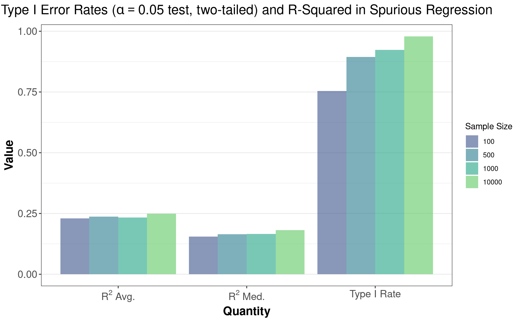
Glancing over the plot above, we can then see that:

We get $R^2$ statistics that are well above zero, which is strange given that the two series are independent.
The true Type-I error rate is between 75 - 97% when using a critical value with a nominal $0.05$ error rate. Thus, we are very likely to make spurious conclusions when regressing two independent, unit-root series on eachother, if we use the traditional critical levels for the hypothesis test.

These results are identical to those found by Granger and Newbold (1974), who note that when using a sample size of 100, “Using the traditional t-test at the 5% level, the null hypothesis of no relationship between the two series would be rejected (wrongly) on approximately three- quarters of all occasions” (115). For the same sample size, the false-rejection rate seen above is the same as stated by the authors.

8.3 Example: Bias of AR(1) Model

In this example I will utlize the steps outlined previously to show that order-1 time-series autoregressive models (AR(1) models) have biased estimators of the autoregressive parameter. This can be shown theoretically, as well, but pretend for the moment that we don’t know such a closed form solution exists, or perhaps we’re too lazy to find one. The Monte Carlo method is well suited for the task.

Briefly, AR(1) models assume a data generating process of the form \[ y_t = \rho y_{t-1} + \varepsilon_t \] where $t = 1, 2, ..., T$ indexes a time period, $|\rho| < 1$, and for the time being we’ll assume that $\varepsilon_t \overset{iid}{\sim} \mathcal{N}(0, 1)$, although with large enough sample sizes normality is not required. Then we can estimate $\rho$ by \[\hat\rho = \frac{\sum_t (y_t - \bar y)(y_{t-1} - \bar y)}{\sum_t (y_{t-1} - \bar y)^2}\] that is, by using its (ordinary) least squares estimator (which is also the sample autocorrelation function).

Using the Monte Carlo method, we will show that $\mathbb{E}(\hat\rho) - \rho \neq 0$, meaning that $\hat\rho$ is biased. In fact, we’ll determine that $|\mathbb{E}(\hat\rho)| < |\rho|$, meaning that the AR parameter is biased towards zero.

In the below, I will simply apply what was discussed in the previous sections without further discussion. The intention here is to give example code for more complicated problems, but the principles in application are identical to those already discussed.

8.3.1 Simulation: Bias of AR(1)

### Install, load default packages (see `Helper Functions`)
inst_load()

### Define AR(1) Simulation function, with intercept
simulation_fn = function(grid_row){
  
  grid_row = unlist(grid_row)
  
  rho = grid_row["p"]
  
  y = list()
  y[[1]] = rnorm(1)
  
  for(j in 2:grid_row["n"]) {
    y[[j]] = rnorm(1, mean = .5 + rho*y[[j-1]])
  }
    
  return(
    data.frame(
      y = unlist(y),
      lag_y = c(NA, head(unlist(y), -1)) # Base lag() function conflicts with dplyr namespace, safest to lag manually
    )
  )
  
}


### Define estimation function
estimation_fn = function(dat, grid_row, iter_id){
  

  mod = lm(y ~ lag_y, data = dat)
  
  return(
    data.frame(iter_id = iter_id, 
               est = coef(mod)[2], 
               n = grid_row[["n"]],
               p = grid_row[["p"]]
               )
    )
  
}


### Define grid
n = c(30, 50, 100, 500, 2500)
p = c(.2, .5, .75, .95)

nsims = 1000
grid = expand.grid(n = n, 
                   p = p
        )
chunks = seq(from = nsims, 
             to = nsims * nrow(grid), 
             by = nsims
          )


### Simulate
setup_cl()

out = 
  foreach(
  i = seq_len(nrow(grid)*nsims),
  .options.multicore = list(preschedule=T),
  .maxcombine = nrow(grid)*nsims,
  .multicombine = T,
  .packages = 'RhpcBLASctl'
) %dorng% {
  
  RhpcBLASctl::blas_set_num_threads(1)
  RhpcBLASctl::omp_set_num_threads(1)
          
  grid_row = grid[which.max(i <= chunks),]
  
  dat = simulation_fn(grid_row)
  
  return(estimation_fn(dat, grid_row, i))
  
}

clear_cl()

8.3.2 Plotting: Bias of AR(1)

### Bind up results and summarize
res = do.call(rbind.data.frame, out)

sums = res %>% 
  dplyr::group_by(n, p) %>% 
  dplyr::summarize(mean_lag = mean(est)) %>% 
  dplyr::mutate(bias = 100*(mean_lag/p - 1))


### Plot
ggplot(sums, aes(y = bias, x = factor(p), fill = factor(n))) +  
  geom_col(position="dodge", alpha = .6) +
  scale_fill_viridis_d(begin = .2, 
                       end = .8, 
                       name = "Sample Size"
                       ) +
  scale_x_discrete(position = "top") +
  theme_bw() + 
  theme(plot.title = element_text(hjust = 0.5, face="bold", size = 17),
        panel.grid.major.x = element_blank(),
        panel.grid.minor.x = element_blank(),
        axis.text = element_text(size=13),
        axis.title=element_text(size=15,face="bold")
        ) +
  labs(x = expression(paste("True Autoregressive Parameter (", rho, ")")),
       y = "% Bias",
       title = "AR(1) Models are Downward Biased")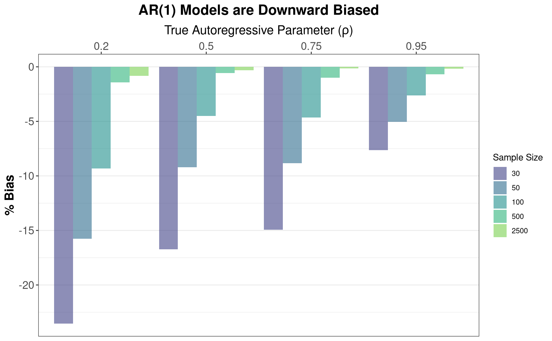

As the plots above show, AR(1) models are indeed biased downward, with this bias abating with increasing sample size. This is particularly informative for Dickey-Fuller tests or other tests for unit roots, as some of these tests implicitly rely on the parameter estimate from an auto-regressive model. In small samples, these parameter estimates are biased downards, implying that we will fail to conclude that the data have a unit-root more frequently, i.e., these tests have low power in small samples, and will have elevated Type II error.

8.4 Example: Censored Regression

For a more complicated set of simulations, I investigate OLS’ performance when the outcome variable is censored, and compare it to both a Heckman 2-step procedure, and a full-information maximum likelihood estimator.

Suppose we have some continuous outcome $y_i^*$, but instead of observing $y_i^*$, we observe $y_i$, defined as \[y_i = \begin{cases} y_i^* \,\, \text{if} \,\, y_i^* > 0 \\ 0 \,\,\,\,\, \text{if} \,\, y_i^* \leq 0 \end{cases} \]

That is, we observe the true value only if it is above some threshold, in this case zero. Otherwise we set $y_i = 0$. This is one form of censoring. We could also delete the observations where we do not observe $y_i^*$, but this would neglect the fact that we may have other information available on that observation.

Now suppose that $y_i^* = \boldsymbol x_i \boldsymbol\beta + \varepsilon_i$, with $\varepsilon \overset{iid}{\sim} \mathcal{N}(\mu, \sigma^2)$. That is, $y_i^*$ is normally distributed, and is a linear function of $\boldsymbol x$ with a well-behaved error term. Given that we don’t observe $y_i^*$, we instead observe $y_i$, we are left to figure out how to estimate a regression model that will recover an unbiased, consistent estimate of the true quantity $\beta$. We’ll consider three approaches here:

Estimating OLS on the observed data, setting unobserved values to zero, which ignores censoring in the data.
Incorporate the probability of censoring into our estimate of the conditional mean, using the Heckman 2-step procedure.
Estimate the regression model using maximum likelihood, specifying a likelihood that accounts for censoring (full-information maximum likelihood, or FIML).

For the sake of brevity, I don’t go into great detail on each approach here, leaving a deeper understanding of each method ``as an exercise,” as they say. However, to get people started in the right direction, a few notes are in order.

A good resource for these items is Long (1997), Ch.7.
The Heckman 2-step procedure accounts for censoring by first estimating the probability of censoring via a probit GLM. The linear predictor from this probit model is then used to estimate the inverse Mills ratio. Finally this estimated inverse Mills ratio is used as an additional “covariate’’ in a second-stage OLS regression on the truncated data. Specifically, $\hat y = X\beta + \hat\gamma \hat \lambda(\hat\eta)$, where $\hat\gamma$ is the slope estimate on the inverse Mills ratio, $\hat\lambda$ which is estimated by evaluating it at $\hat\eta$, the linear predictor from the first-stage probit.
The FIML estimator just specifies a likelihood for the generation of both censored and uncensored data, and maximizes it in the usual way. Specifically, \[L(\beta, \sigma^2 | y, X) = \prod_{obs} \frac{1}{\sigma}\phi\left(\frac{y - X\beta}{\sigma}\right) \prod_{cens} \Phi\left(\frac{\tau - X\beta}{\sigma}\right)\] where:
- $\phi$ is the p.d.f. of the standard normal distribution,
- $\Phi$ is the c.d.f. of the standard normal distribution,
- $\tau$ is the censoring threshold; in the case above, this is $\tau = 0$.
- $cens$ indicates that the portion of the likelihood is for censored observations.
- $obs$ indicates that the portion of the likelihood is for uncensored observations.

From this we can see that FIML is just composed of a normal linear model’s likelihood for the observed data, and the probability of censoring for the censored data. We can then take logs and maximize the resulting log-likelihood as usual. This is done in the below code.

8.4.1 Simulation: Censored Regression

### Install and load necessary packages (see `Helper Functions`)
inst_load()


### FIML likelihood function
fiml_ll = function(parms,  y, X, tau = 0){
  
  b = head(parms, -1)
  sig = tail(parms, 1)

  obs =  y > tau
  
  y_obs = y[obs]
  y_cen = y[!obs]
  eta = as.vector(X %*% b)
  eta_obs = eta[obs]
  eta_cen = eta[!obs]
  
  ll_uncens = sum(dnorm((y_obs - eta_obs)/sig, log=T) - log(sig))
  ll_cens = sum(pnorm((tau - eta_cen)/sig, log.p = T))
  
  ll = -(ll_uncens + ll_cens)
  
  return(ll)
  
}


### Define custom FIML regression function
fiml_reg = function(formula, data, ...){
  
  fr = model.frame(formula, data = data)
  X = model.matrix(formula, fr)
  y = model.response(fr)
  
  starts = c( 
    coef(lm(y ~ X + 0)),
    1
  )
  
  mod = nlm(fiml_ll, p = starts, hessian = T, X=X, y = y, ...)
  se = sqrt(diag(solve(mod$hessian)))

  out = cbind.data.frame(est = mod$estimate, se = se)
  return(out)
  
}


### Simulation function
simulation_fn = function(grid_row, b) {
  n = grid_row[["n"]]

  X = cbind(
    1, 
    rnorm(n, sd = 2.5)
  )
  
  y = rnorm(n, mean = X%*%b, sd = 1.75)

  obs =  as.integer(y > 0)
  y[obs == 0] = 0
  
  out = cbind.data.frame(
    X = X, 
    y = y, 
    obs = obs
  )
  
  return(out)
    
}


### Estimation function
estimation_fn = function(dat, grid_row, iter, b){
  n = grid_row[,"n"]
  grid_row = unname(unlist(grid_row)) # to avoid naming conflicts later
  
  
  # Model 1 - OLS
  ols = lm(y ~ X.2, data = dat)
  
  
  # Model 2 - Heckman
  hecksel = suppressWarnings(
    glm(
      obs ~ X.2,
      family = binomial(link = "probit"),
      data = dat
    )
  )
  
  eta = predict(hecksel)
  
  imills = dnorm(eta)/pnorm(eta)
  
  heck2step = lm(y ~ X.2 + imills,
                 data = dat,
                 subset = obs == 1
                 )
  
  
  # Model 3 - FIML Tobit 1
  out_fiml = fiml_reg(y ~ X.2, data = dat, iterlim = 5000)[1:2,]
  
  
  # Proportion observed, tells how censored 
  prop_obs = sum(dat$obs) / nrow(dat)
  
  
  # Tidy everything for clean results
  out_2step = summary(heck2step)$coefficients[1:2, 1:2]
  out_ols = summary(ols)$coefficients[1:2, 1:2]
  
  colnames(out_2step) = colnames(out_ols) = colnames(out_fiml) =  c("est", "se")
  rownames(out_2step) = rownames(out_ols) = rownames(out_fiml) = c("b1", "b2")

  model = rep(c("ols", "2step", "fiml"), each = nrow(out_2step))

  out = cbind.data.frame(
    model = model,
    rbind.data.frame(out_ols, out_2step, out_fiml)
  )

  rownames(out) = NULL
 
  data.frame(
    iter_id = iter,
    param = rep(rownames(out_2step), 3),
    b1 = unname(b["b1"]),
    b_tru = rep(unname(b), 3),
    n = n,
    prop_obs = prop_obs,
    out
  )
  
} ### End Estimation function


### Set up for simulations
n = c(50, 500, 5000)
b1 = c(1, 2, 3)

nsims = 1000
grid = expand.grid(n = n, 
                   b1 = b1
        )
chunks = seq(from = nsims, 
             to = nsims*nrow(grid), 
             by = nsims
          )


### Main simulations
setup_cl()

out = 
  foreach(
  i = seq_len(nrow(grid)*nsims),
  .options.multicore = list(preschedule=T),
  .maxcombine = nrow(grid)*nsims,
  .multicombine = T,
  .packages = c('RhpcBLASctl')
) %dorng% {
  
  RhpcBLASctl::blas_set_num_threads(1)
  RhpcBLASctl::omp_set_num_threads(1)
          
  grid_row = grid[which.max(i <= chunks),]
  
  b1 = grid_row[["b1"]]
  b = c(b1 = b1, b2 = -1.75)
  
  dat = simulation_fn(grid_row, b)
  
  estimation_fn(dat, grid_row, i, b)
  
}
  
clear_cl()

8.4.2 Plotting: Censored Regression

### Bind up the results list into a data.frame
res = do.call(rbind.data.frame, out)

### Summarize the data for plotting
sums = res %>% 
  dplyr::group_by(b1) %>%
  dplyr::mutate(avg_obs = round(mean(prop_obs),2),
                est_c = 100*(est - b_tru)/b_tru
  )


### Re-order brewer color palette so that green is the "best" model in plots
clrs = RColorBrewer::brewer.pal(3, "Set1")[c(2,3,1)]

### Plot Intercept, showing upward bias
ggplot(sums[sums$param == "b1",], aes(x = est_c, fill = model, color = model)) + 
  geom_density(trim = T, alpha = .25, bw = "SJ") +
  scale_fill_manual(labels =  c("2-Step", "FIML", "OLS"),
                    values = clrs) +
  scale_color_manual(labels =  c("2-Step", "FIML", "OLS"),
                     values = clrs) +
  geom_vline(xintercept = 0, lty = "dashed") +
  facet_grid(avg_obs ~ n,
             labeller = label_bquote(
               rows = "Prop. Observed" == .(avg_obs),
               cols = "n" == .(n)
              )) + 
  coord_cartesian(xlim = c(-35, 150)) +
  labs( x = expression(paste("% Difference  (", hat(beta)-beta,")/", beta)),
        y = "Kernel Density Estimate",
        title = "The Intercept is Biased Upwards Under Censoring, and 2-Step is Inefficient" ) +
  theme_bw() + 
  theme(plot.title = element_text(hjust = 0.5, face="bold", size = 17),
        axis.text = element_text(size=13, face = "bold"),
        axis.title=element_text(size=15,face="bold"),
        strip.text = element_text(size = 12, face = "bold")
        )

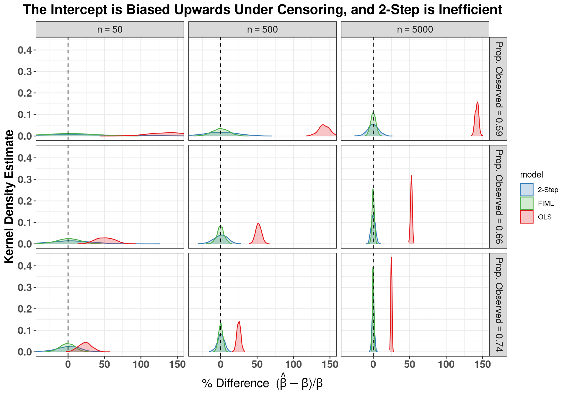
### Plot slope, showing downward bias
ggplot(sums[sums$param == "b2",], aes(x = est_c, fill = model, color = model)) + 
  geom_density(trim = T, alpha = .25, bw = "SJ") +
  scale_fill_manual(labels =  c("2-Step", "FIML", "OLS"),
                    values = clrs) +
  scale_color_manual(labels =  c("2-Step", "FIML", "OLS"),
                     values = clrs) +
  geom_vline(xintercept = 0, lty = "dashed") +
  facet_grid(avg_obs ~ n,
             labeller = label_bquote(
               rows = "Prop. Observed" == .(avg_obs),
               cols = "n" == .(n)
              )) + 
  coord_cartesian(xlim = c(-60, 15)) +
  labs( x = expression(paste("% Difference  (", hat(beta)-beta,")/", beta)),
        y = "Kernel Density Estimate",
        title = "The Slope is Biased Downwards Under Censoring, and 2-Step is Inefficient" ) +
  theme_bw() + 
  theme(plot.title = element_text(hjust = 0.5, face="bold", size = 17),
        axis.text = element_text(size=13, face="bold"),
        axis.title=element_text(size=15,face="bold"),
        strip.text = element_text(size = 12, face = "bold")
        )

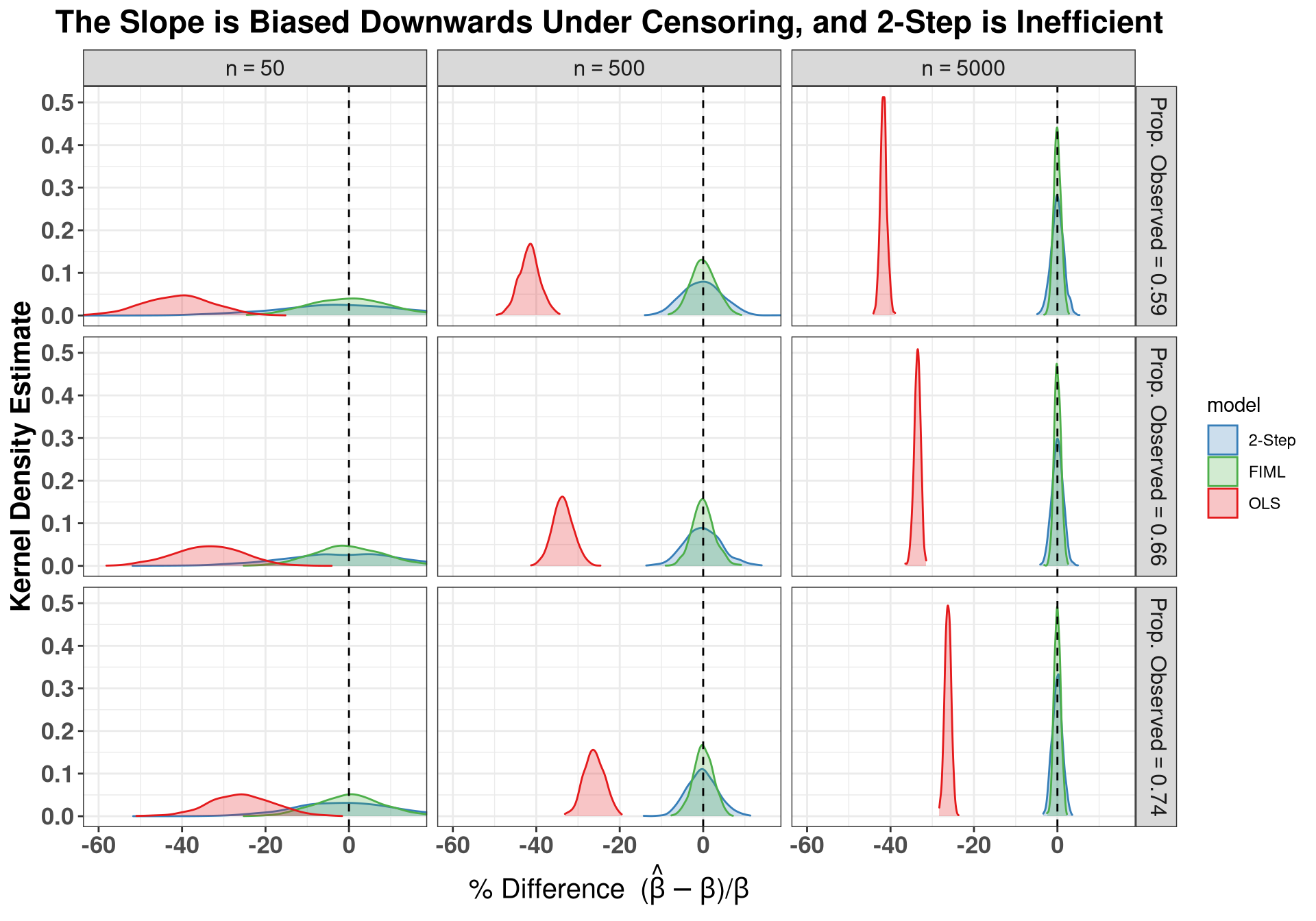
Briefly, we can make three primary conclusions from the above plots:

OLS intercepts are biased upward, while the slope is biased downwards in the presence of censoring.
The Heckman 2-step procedure is unbiased for both the intercept and slope.
FIML regression is unbiased, and is more efficient than the Heckman procedure. This makes sense, as the Heckman model has less data, and treats the Mills ratio as if it isn’t also a random variable, when in fact it is. Thus, if using the Heckman, bootstrapping standard errors would be necessary.

8.5 Example: Bias of Logistic Regression

Finally, the Monte Carlo methods presented here are applied to the case of logistic regression, specifically to show that logistic regression coefficients are biased upwards in small samples, and to show that one solution to this is to add a penalty to the likelihood function as a correction.

For references on the subject, see Firth (1993), Rainey and McCaskey (2021), and the R-package brglm2.

If you are familiar with ridge regression or Least Angular Shrinkage and Selection Operator (LASSO) regression, the intuition of Firth (1993) is similar: we add a penalty to the log-loss function that is increasing in some norm of the coefficients, which causes us to push coefficients towards zero. Because logistic regression coefficients are biased upwards in small samples, pushing them a bit towards zero is what we need for unbiasedness.

8.5.1 Simulation: Bias of Logistic Regression

### Install, load necessary packages (see `Helper Functions`)
inst_load(pks = 'brglm2')


### Define Simulation function
simulation_fn = function(grid_row){
  b1 = grid_row[["b1"]]
  n = grid_row[["n"]]
  btrue = grid_row[["btrue"]]
  
  X = cbind(
    1,
    rexp(n, .25),
    matrix(rnorm(n * 4), ncol=4)
    )
  
  b = c(b1, btrue, 1.75, -.25, .5, -2.33)
  eta = X%*%b
  
  y = rbinom(n, 1, plogis(eta))
  
  dat = cbind.data.frame(y = y, X = X[,-1])
  
  return(dat)
}

### Define Estimation Function
estimation_fn = function(data, grid_row, iter_id){
  
  grid_row = unlist(grid_row)
  
  # Model 1 - ML logit, filter out perfect prediction/non-convergence 
  mod_bad = tryCatch(
    glm(y ~ . , 
        data = dat, 
        family=binomial(link="logit")
      ), 
    warning = function(w) if(grepl("fitted probabilities || not converge", w$message)) return(NULL) else warning(w$message)
  )

  
  if(is.null(mod_bad))
    return(NULL)
  
  # Model 2 - PML "Firth" Logit
  mod_good = glm(y ~ . , 
                 data = dat,
                 method = "brglmFit",
                 type = 'AS_mean',
                 family = binomial(link = "logit")
              )
  
  # Get proportion of successes in model
  success = mean(dat$y)
  
  # Get coefs
  out_bad = summary(mod_bad)$coefficients[2, 1:2]
  out_good = summary(mod_good)$coefficients[2, 1:2]
  
  out = rbind(out_bad, out_good)
  colnames(out) = c("est", "se")
  
  cbind.data.frame(
    iter_id = iter_id,
    n = grid_row[["n"]],
    b1 = grid_row[["b1"]],
    success = success,
    btrue = grid_row[["btrue"]],
    model = c("ML", "PML"),
    out
  )

}


### Set up Simulations
nsims = 1000
b1 = 2:5
n = c(50, 100, 150, 200, 500)
grid = expand.grid(b1 = b1, 
                   n = n
        )

# True Slope coefficient (invariant)
grid$btrue = -.75

chunks = seq(from = nsims, 
             to = nsims*nrow(grid), 
             by = nsims
          )


### Do simulations
setup_cl()

out = 
  foreach(
    i = seq_len(nrow(grid)*nsims),
    .options.multicore = list(preschedule=T),
    .maxcombine = nrow(grid)*nsims,
    .multicombine = T,
    .packages = c('RhpcBLASctl', 'brglm2')
) %dorng% {
  
  
  library(brglm2)
  RhpcBLASctl::blas_set_num_threads(1)
  RhpcBLASctl::omp_set_num_threads(1)
          
  stopifnot(i >= 1 && i <= tail(chunks, 1))
  grid_row = grid[which.max(i <= chunks),]
  
  dat = simulation_fn(grid_row)
  summary(dat)
  
  estimation_fn(dat, grid_row, i)
  
}
  
clear_cl()

8.5.2 Plotting: Bias of Logistic Regression

### Bind everything up
res = do.call(rbind.data.frame, out)


### Add in percent difference (est_c) and compute average success rate (affected by intercept)
res$est_c = 100*(res$est - res$btrue)/res$btrue
res = res %>% 
  group_by(b1) %>% 
  mutate(success = round(mean(success), 2)) %>%
  group_by(n, b1, btrue, model) %>%
  mutate(avg = mean(est_c))


### Group level summaries for bar plots
sums = res %>%
  group_by(b1) %>% 
  mutate(success = round(mean(success), 2)) %>%
  group_by(n, success, btrue, model) %>%
  mutate(reject = abs(est/se) > qnorm(.975)) %>%
  summarise(avg = mean(est),
            power = mean(reject)) %>% 
  mutate(bias = 100*(avg - btrue)/btrue)


### Density Plots
ggplot(res, aes(x = est_c, fill = model, color = model)) +
  geom_density(trim = T, alpha = .15, bw = "SJ") +
  scale_fill_brewer(palette = "Set1") +
  scale_color_brewer(palette = 'Set1') +
  facet_grid(success ~ n,
             labeller = label_bquote(
               rows = "Prop. Success" == .(success),
               cols = "n" == .(n)
              )) + 
  coord_cartesian(xlim = c(-100, 150)) +
  geom_vline(data = res, 
             aes(xintercept = avg, color = model), 
             lty = "dashed") + 
  geom_vline(xintercept = 0, lty = 'dotted') + 
  labs(
      x = expression(paste("% Difference  (", hat(beta)-beta,")/", beta)),
      y = "Kernel Density Estimate",
      title = "PML Models are Less Biased, More Efficient than ML Logit Models with small N"
  ) +
  theme_bw() + 
  theme(plot.title = element_text(hjust = 0.5, face="bold", size = 17),
        axis.text = element_text(size=10),
        axis.title=element_text(size=15,face="bold"),
        strip.text = element_text(size = 12, face = "bold")
        )

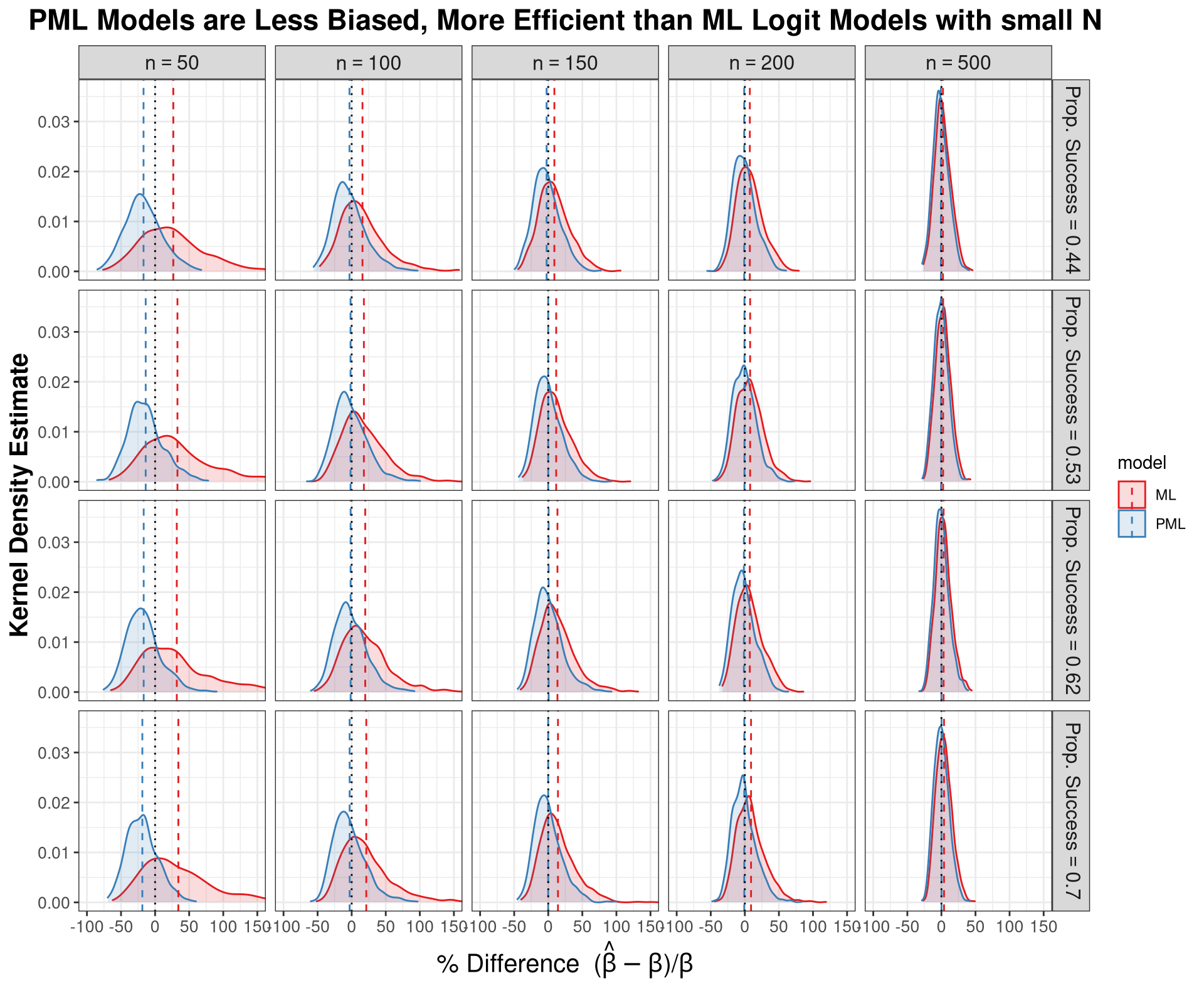
### Barplot for Bias
ggplot(sums, aes(y = bias, x = factor(model), fill = factor(n))) +  
  geom_col(position="dodge", alpha = .6) +
  scale_fill_viridis_d(begin = .2, 
                       end = .8, 
                       name = "Sample Size"
                       ) +
  facet_wrap(vars(success),
             labeller = label_bquote("Prop. Success" == .(success))) +
  labs(
    x = "Model",
    y = "% Bias",
    title = "PML Logit Models are Less Biased than ML Logit Models"
  ) +
  theme_bw() + 
  theme(plot.title = element_text(hjust = 0.5, face="bold", size = 17),
        panel.grid.major.x = element_blank(),
        panel.grid.minor.x = element_blank(),
        axis.text = element_text(size=13, face = "bold"),
        axis.title=element_text(size=15,face="bold"),
        strip.text = element_text(size = 12, face = "bold")
        )

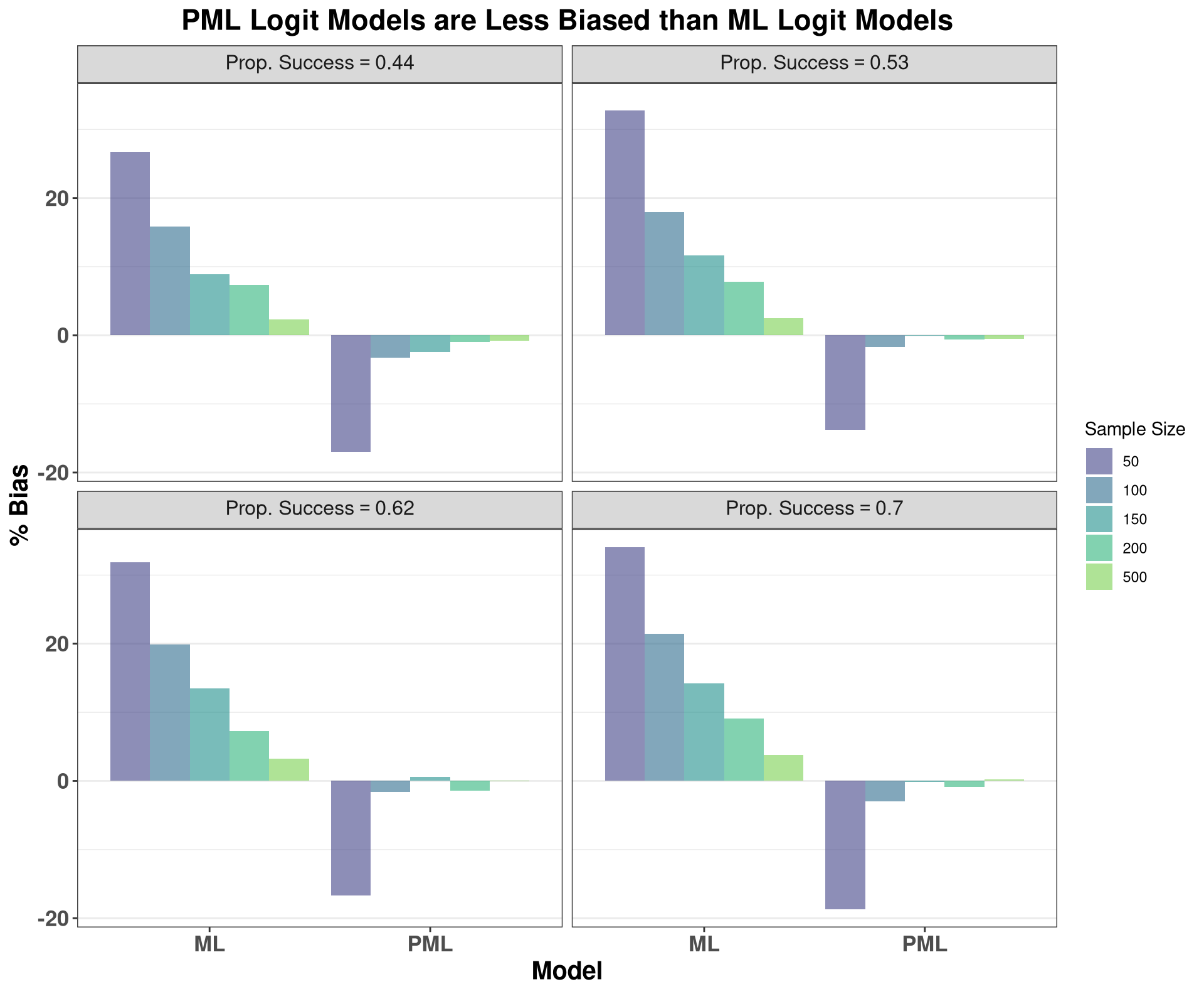
### Barplot for power
ggplot(sums, aes(y = power, x = factor(model), fill = factor(n))) +  
  geom_col(position="dodge", alpha = .6) +
  scale_fill_viridis_d(begin = .2, 
                       end = .8, 
                       name = "Sample Size"
                       ) +
  facet_wrap(vars(success),
             labeller = label_bquote("Prop. Success" == .(success))) +
  labs(
    x = "Model",
    y = "Power",
    title = "PML Logit Models Retain Power Despite Downward Bias"
  ) +
  theme_bw() +
  theme(plot.title = element_text(hjust = 0.5, face="bold", size = 17),
        panel.grid.major.x = element_blank(),
        panel.grid.minor.x = element_blank(),
        axis.text = element_text(size = 13, face = "bold"),
        axis.title=element_text(size = 15,face="bold"),
        strip.text = element_text(size = 12, face = "bold")
        )

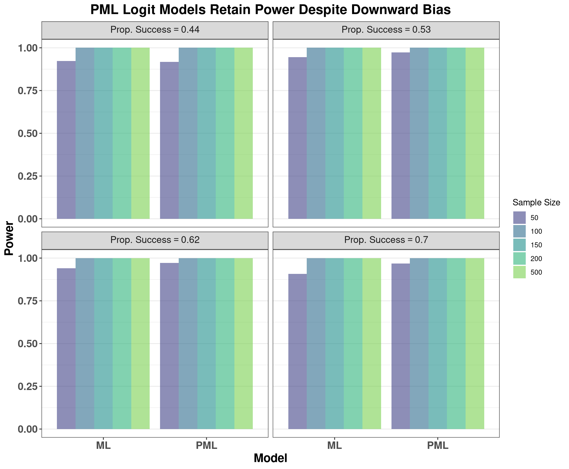
Briefly describing the above plots, I vary the intercept of the data generating process in order to affect the proportion of successes and failures in the data, which affects the estimator. The average number of sucesses over all simulations for that value of the intercept is then used to label the proportion of successes in each plot.

In the density plots we can clearly see that the PML estimator has lower variance than the naive logistic model in small samples, but that this reduction abates as we get more data. It is hard to establish the bias of each estimator using the density plots, but I’ve drawn dashed vertical lines to denote the mean of each distribution. However, below the density plots we can directly see the percent bias explicitly in the bar plot. In very small samples, the PML estimator is over aggressive, so the coefficients actually end up biased downward. However, in all other cases, it is substantially less biased than the naive logistic model.

Because we are pushing the coefficients towards zero, we may be fearful that our type II error rates may go up, i.e., that the model loses power. However, because of the simultaneous reduction in variance (meaning there is no bias-variance tradeoff, as noted in the citations provided earlier), it turns out that the shrinkage of the coefficients does not result in lower power, as seen in the third plot (or second set of bar plots).

Long, J Scott. 1997. “Regression Models for Categorical and Limited Dependent Variables.” Advanced Quantitative Techniques in the Social Sciences 7.

This is in fact the biased sample variance. Despite being biased, it is still weakly consistent/convergent. So as not to confuse readers, I did not delve into the biased sample variance, as it does not admit a simple “sample mean” formulation (i.e., 1/n…) without some manipulation. Note however that the unbiased sample variance also does converge in probability to the true mean, i.e., it is consistent.↩︎
Here I use a kernel-based estimator of the density function to highlight its interpretation as a sample mean. However, other estimators exist which are consistent for the population density function.↩︎
This is a simplistic sample estimator of the quantile function, used here primarily for presentation purposes. In reality, other estimators exist that are superior, and are still weakly consistent/convergent.↩︎
I’m aware that multi-threading and parallelism are not the same thing. To keep things simple I treat them as the same here, as their difference is not relevant for explaining the issue here.↩︎

Monte Carlo Analysis in R: An in Depth Guide, with Examples

Updated: 10 Oct 2022

1 Brief Review of Monte Carlo Methods

2 Simulations: Serial vs Parallel

2.1 Differences between `foreach` and `for`

2.2 Making `foreach` Run in Parallel

2.3 Important `foreach` Parameters

2.4 `FORK` or `PSOCK`?

3 Seed Setting and Parallelism

3.1 Option 1: `doRNG`

3.2 Option 2: Iteration-level Seeds

4 Thread Competition

4.1 BLAS/LAPACK-Induced Deadlock

4.2 Multi-threaded Packages

4.3 Solving Thread Competition

4.4 Caveats

5 Parameter Grids

5.1 Extending Grids to Multiple Simulations

5.2 Why not use a nested loop?

5.3 Caveats

6 Using Functions Properly

6.1 Simulation Function

6.2 Estimation Function

7 Things You Should and Shouldn’t Do

8 Examples

8.1 Extremely Useful Functions

8.2 Example: Spurious Regression

8.2.1 Simulation: Spurious Regression

8.2.2 Plotting: Spurious Regression

8.3 Example: Bias of AR(1) Model

8.3.1 Simulation: Bias of AR(1)

8.3.2 Plotting: Bias of AR(1)

8.4 Example: Censored Regression

8.4.1 Simulation: Censored Regression

8.4.2 Plotting: Censored Regression

8.5 Example: Bias of Logistic Regression

8.5.1 Simulation: Bias of Logistic Regression

8.5.2 Plotting: Bias of Logistic Regression

Monte Carlo Analysis in R: An in Depth Guide, with Examples

Updated: 10 Oct 2022

1 Brief Review of Monte Carlo Methods

2 Simulations: Serial vs Parallel

2.1 Differences between foreach and for

2.2 Making foreach Run in Parallel

2.3 Important foreach Parameters

2.4 FORK or PSOCK?

3 Seed Setting and Parallelism

3.1 Option 1: doRNG

3.2 Option 2: Iteration-level Seeds

4 Thread Competition

4.1 BLAS/LAPACK-Induced Deadlock

4.2 Multi-threaded Packages

4.3 Solving Thread Competition

4.4 Caveats

5 Parameter Grids

5.1 Extending Grids to Multiple Simulations

5.2 Why not use a nested loop?

5.3 Caveats

6 Using Functions Properly

6.1 Simulation Function

6.2 Estimation Function

7 Things You Should and Shouldn’t Do

8 Examples

8.1 Extremely Useful Functions

8.2 Example: Spurious Regression

8.2.1 Simulation: Spurious Regression

8.2.2 Plotting: Spurious Regression

8.3 Example: Bias of AR(1) Model

8.3.1 Simulation: Bias of AR(1)

8.3.2 Plotting: Bias of AR(1)

8.4 Example: Censored Regression

8.4.1 Simulation: Censored Regression

8.4.2 Plotting: Censored Regression

8.5 Example: Bias of Logistic Regression

8.5.1 Simulation: Bias of Logistic Regression

8.5.2 Plotting: Bias of Logistic Regression

2.1 Differences between `foreach` and `for`

2.2 Making `foreach` Run in Parallel

2.3 Important `foreach` Parameters

2.4 `FORK` or `PSOCK`?

3.1 Option 1: `doRNG`